An Improved Lower Bound for Non-Anytime Gradient Descent
Introduction
Last week, Ma and Chen established an \(\Omega(n^{-1.932})\) lower bound for non-anytime gradient descent (GD) under arbitrary non-adaptive stepsize schedules in smooth convex optimization. Since I have been constantly thinking about this problem, I was very excited to see this result. As the paper is not easy to follow, I spent some time understanding and verifying the proof myself with the help of ChatGPT-5.6. The goal of this blog post is to
- Explain the construction of the hard functions in Ma and Chen;
- Improve the lower bound for non-anytime GD to \(\Omega(n^{-\sqrt{3}})\).
I hope this blog post will be helpful to the community, and I would appreciate any comments. A preprint covering the results will be released soon.
AI Disclosure: The improvement was made by ChatGPT-5.6 Sol with minimal human guidance. However, the generated proof is difficult to follow, so it took me several days to simplify and rewrite it. The blog post was first written solely by me and then revised by ChatGPT.
Problem Setup
Let \(\mathcal{F}_1(\mathbb{R}^d)\) denote the class of \(1\)-smooth convex functions on \(\mathbb{R}^d\) whose sets of minimizers are nonempty. Consider non-anytime GD for minimizing a smooth convex function \(f\in\mathcal{F}_1(\mathbb{R}^d)\): $$x^\star \in \arg\!\min_{x\in\mathbb{R}^d}f(x).$$ Given an initial point \(x_1\in\mathbb{R}^d\) and a stopping time \(n\in\mathbb{N}\), non-anytime GD generates the iterates by following the update rule: $$x_{k+1} = x_k - h_k \nabla f(x_k), \quad\forall k\in[n],$$ where \([n]:=\{1,2,\ldots,n\}\) and \(H:=(h_1,\ldots,h_n)\in(0,\infty)^n\) is a stepsize schedule that may depend on \(n\) but does not depend on \(f\). For a stopping time \(n\in\mathbb{N}\) and a stepsize schedule \(H\in(0,\infty)^n\), the (worst-case) convergence rate is defined as $$R_n(H) := \sup_{d\in\mathbb{N}} \sup_{f\in\mathcal{F}_1(\mathbb{R}^d)} \sup_{x^\star\in\arg\!\min f}\sup_{ x_1\in\mathbb{R}^d } \frac{ f(x_{n+1}) - f(x^\star) }{ \frac{1}{2}\lVert x_1 - x^\star \rVert^2 }.$$ We say that non-anytime GD can achieve a convergence rate of order \(O(\varphi(n))\) if there exists a constant \( c>0\) such that for every stopping time \(n\in\mathbb{N}\), there exists a stepsize schedule \(H^{(n)}\in(0,\infty)^n\) such that \(R_n(H^{(n)}) \leq c\varphi(n)\).
Main Results
The following theorem is the main result of Ma and Chen.
Theorem 1. (Ma and Chen) Let \(p^\ast = \sqrt{2+\sqrt{3}}\approx 1.9319\). For every \(p\in(p^\ast,2)\), there exists a constant \(c_p>0\) such that for any \(n\in\mathbb{N}\) and any \(H\in(0,\infty)^n\), \(R_n(H) \geq c_pn^{-p}\). Therefore, non-anytime GD cannot achieve a convergence rate of order \(O(n^{-1.932})\).
In this blog post, we will prove the following theorem. It improves Theorem 1 and is the current best known lower bound.
Theorem 2. There exists a universal constant \(c>0\) such that for any \(n\in\mathbb{N}\) and any \(H\in(0,\infty)^n\), \(R_n(H) \geq cn^{-\sqrt{3}}\). Therefore, non-anytime GD cannot achieve a convergence rate of order \(o(n^{-\sqrt{3}})\).
To better appreciate the above lower bounds, we briefly review some prior work. For more than fifty years, the best convergence rate of GD was widely believed to be \(O(n^{-1})\), which is fundamentally slower than accelerated methods (Nesterov) that achieve the full \( O(n^{-2}) \) accelerated rate. In a breakthrough result three years ago, Altschuler and Parrilo and Grimmer et al. showed that it is possible to break the \(O(n^{-1})\) upper bound by using carefully designed stepsize schedules. This opens the possibility of achieving the \( O(n^{-2}) \) accelerated rate with non-anytime GD.
Since then, proving or disproving the \( O(n^{-2}) \) accelerated rate for GD has been an active research problem. My collaborators and I resolved the problem for anytime GD this year, showing that achieving the \( O(n^{-2}) \) rate is impossible. However, our technique is provably insufficient to resolve the problem for non-anytime GD.
The importance of Theorem 1 is that it settles the question for non-anytime GD.
Although there remains a large gap between the best known upper and lower bounds, Theorem 1 is still a significant breakthrough.
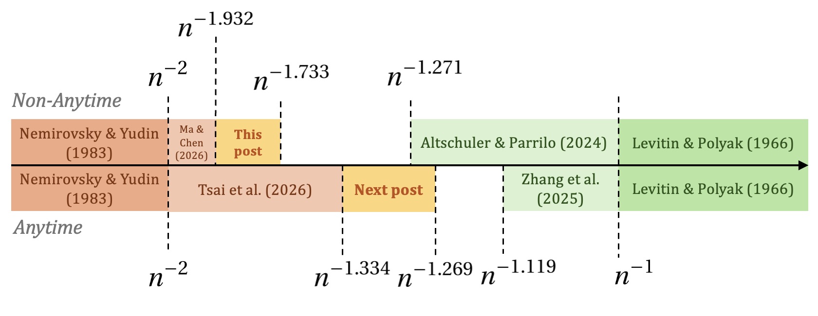
The following figure summarizes our current understanding of the convergence rate of GD.
The optimal rate of non-anytime GD lies between \(\Omega(n^{-1.733})\) and \(O(n^{-1.271})\).
We will discuss the lower bound for anytime GD in the next post.
Since the progress is so fast and the upper and lower bounds match now (see the recent work of Ye and Liu and references therein), I will not to write a post for anytime GD.
Proof Strategy of Theorem 2
We motivate the analysis from the following simple bound. For a sequence \(\{ a_k\}\), we write \(a_{m:n} = \sum_{k=m}^n a_k\) if \(m\leq n\) and define \(a_{m:n}=0\) if \(n<m\).
Lemma 3 (Huber functions, see, e.g., Grimmer et al.). For any \(n\in\mathbb{N}\) and any \(H=(h_1,\ldots,h_n)\in(0,\infty)^n\), we have $$R_n(H) \geq \frac{1}{2h_{1:n}+1}.$$
By Lemma 3, any upper bound on the sum of all stepsizes \(h_{1:n}\) directly implies a lower bound on the convergence rate. This suggests the strategy of proving upper bounds on the number and the magnitude of large stepsizes in \(H\). The proof can therefore be divided into two main parts, which we explain in more detail in the following sections.
- In the first part, we construct a family of high-dimensional functions such that if \(H\) contains many large stepsizes, then GD does not perform well. This family of hard functions was first constructed by Ma and Chen.
- In the second part, we extract properties of a good stepsize schedule from these hard functions. In particular, we establish an upper bound on the number of large stepsizes in \(H\).
Finally, we bound the sum \(h_{1:n}\) and complete the proof by Lemma 3.
The Hard Functions of Ma and Chen
To upper bound the number and the magnitude of large stepsizes, Ma and Chen constructed hard functions \(f\) such that \(R_n(H)\) is large if \(H\) contains too many large stepsizes. Conversely, if \(R_n(H)\) is small, then \(H\) should not have many large stepsizes. We first go through some motivating examples in existing works.
Generalized Huber Functions
The hard functions we construct in the following have the following form: $$\tag{1}f(x) = \frac{1}{2}\lVert x\rVert^2 - \frac{1}{2}d(x,C)^2, \quad x\in\mathbb{R}^d,$$ where \(C\subseteq\mathbb{R}^d\) is a closed convex set such that \(0\in C\) and \(d(x,C):=\displaystyle\min_{c\in C}\lVert x-c\rVert\) is the distance between a point \(x\) and the set \(C\). Since these functions cover the Huber function by taking \(d=1\) and \( C=[-\delta,\delta] \) for some \(\delta>0\), we call them the generalized Huber functions. In addition, they also cover the quadratic function by taking \(C=\mathbb{R}^d\), and the hard functions used to establish the non-acceleration of Polyak's heavy-ball method. The functions (1) are \(1\)-smooth convex, quadratic inside \(C\), and minimized by \(0\). Furthermore, we have \( \nabla f(x) = \Pi_C(x) \) for every \( x\in\mathbb{R}^d\), where \(\Pi_C\) is the orthogonal projection onto \(C\). See, e.g., Corollary 12.31 of Bauschke and Combettes. This provides a nice geometric picture of the functions.
Penalizing One Large Step
When there is one extremely large stepsize, my collaborators and I generalized the construction of Kornowski and Shamir and proved the following lemma.
Lemma 4 (Lemma 3.1 of Tsai et al.) For any \(n\in\mathbb{N}\), any \(H\in(0,\infty)^n\), and any \(m\in[n]\) such that \(h_m>1\), we have $$ R_n(H) \geq \frac{ (h_m-1)^2 }{ (h_{1:m-1} + 1)^2(2h_{m+1:n} + 1) }. $$
We take \(d=1\), \(x_1=1\), and \(C=[-\varepsilon,\delta]\) for some properly chosen \(\varepsilon>0\) and \(\delta>0\) to enforce the following trajectory of GD:
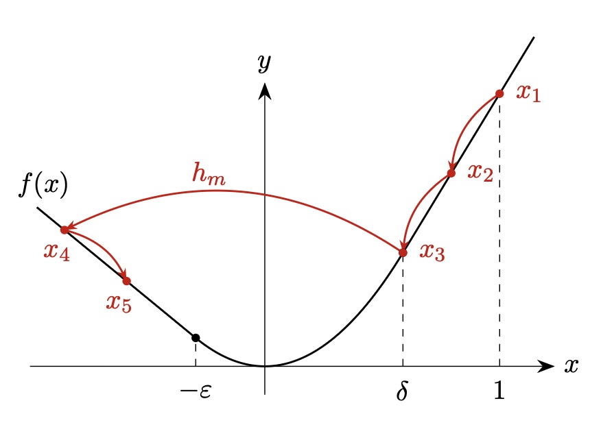
When using the large step \(h_m\), GD "overshoots" to the left side of the minimizer. For all the other steps, GD stays in the same affine part as in the previous iterate.
Penalizing Two Large Steps
Suppose there are two large stepsizes, say \(h_{m}\) and \(h_{n}\). As a first attempt, one may try the same hard functions in Lemma 4 and consider the following trajectory:
- \(\eta_m\) overshoots to the left: \( x_{m+1} < 0 < \delta \leq x_m < \cdots < x_2 < x_1 = 1 \).
- \(\eta_n\) overshoots back to the right: \( x_{m+1} < \cdots < x_n \leq -\varepsilon < 0 < x_{n+1} \).
However, this is not, in fact, the hardest function we can come up with. Ideally, we want \( f(x_{n+1}) \) to be large, but this value depends on \(\delta\), which depends on \( h_{1:m-1} \) in the above construction. In the good case where \(\delta\) is large enough that \( x_{n+1} \leq \delta \), \( f(x_{n+1}) \) grows quadratically in \( h_n\) as in Lemma 4. However, in the bad case where \(\delta\) is small, \( f(x_{n+1}) \) only grows linearly in \( h_n\). The fundamental issue here is that \(\mathbb{R}\) only has one degree of freedom, and we need to go beyond one dimension.
There are several ways to come up with new hard functions. One systematic approach is to study the output of the performance estimation problem (PEP). I won't go into the details of PEP, but the important point here is that PEP can compute the worst functions for every given stepsize schedule numerically. We present the following lemma to illustrate the benefit of constructing high-dimensional functions.
Lemma 5 (My unpublished note). For any \(n\in\mathbb{N}\) such that \(h_{n-1}>3+2\sqrt{2}\) and \(h_n\geq 4\), we have $$ R_n(H) \geq \frac{ (h_{n-1}-1)^2(h_n-1-\sqrt{2h_n+1}) }{(h_{1:n-2}+1)^2}. $$
We take \(d=2\) and \(x_1=(1,0)\). We choose \(C\subseteq\mathbb{R}^2\) to enforce the following trajectory of GD:
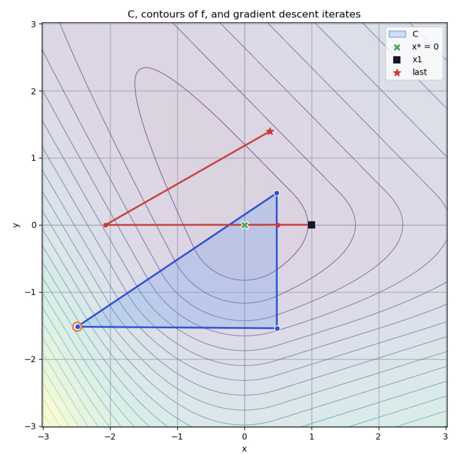
For the \((n-1)\)-th step, GD overshoots to the other side but remains on the \(x\)-axis. For the \(n\)-th step, GD overshoots in a different direction, thanks to the extra degree of freedom in \(\mathbb{R}^2\).
Penalizing Multiple Large Steps
To go beyond two large stepsizes, it is reasonable to construct functions in more than two dimensions. However, from my experience in proving Lemma 5, it is highly nontrivial to come up with functions that are both analytical tractable and hard enough. Ma and Chen succeeded in constructing such functions, and the following lemma is their key result.
Lemma 6 (Theorem 4.1 of Ma and Chen). Fix any \(n\in\mathbb{N}\) and any \(H\in(0,\infty)^n\).
- For \(m\in[n]\), let \(0<t_1<\cdots<t_m \leq n\) be any \(m\) indices such that \(h_{t_i}>1\) for all \(i\in[m]\). Let \(t_0=0\) and \(t_{m+1}=n+1\).
- For \(i\in[m+1]\), let \(S_i = h_{t_{i-1}+1: t_i - 1}\) denote the sum of stepsizes between the chosen \(m\) stepsizes.
Then, we have $$R_n(H) \geq \frac{1}{S_m + h_{t_m} + 2S_{m+1} + 1} \prod_{i=1}^{m-1} \frac{ S_{i+1} + h_{t_{i+1}}}{ S_{i} + h_{t_i} + S_{i+1} + h_{t_{i+1}} } \prod_{i=1}^m \frac{ h_{t_i} - 1 }{ S_i + 1 }.$$ The hard instance \(f\) depends on \(H\) and is supported on \(\mathbb{R}^{m+1}\).
Lemma 6 is the most important lemma in the proof of Theorem 2, and the remaining steps amount to extracting more interpretable information from Lemma 6. The important property of Lemma 6 is that the lower bound increases as \(\{ h_{t_i} \}\) increases, and decreases as \(\{S_i\}\) increases. Therefore, if \(R_n(H)\) is small, then \(m\) and \(\{h_{t_i}\}\) should be small, while \(\{S_i\}\) should be large.
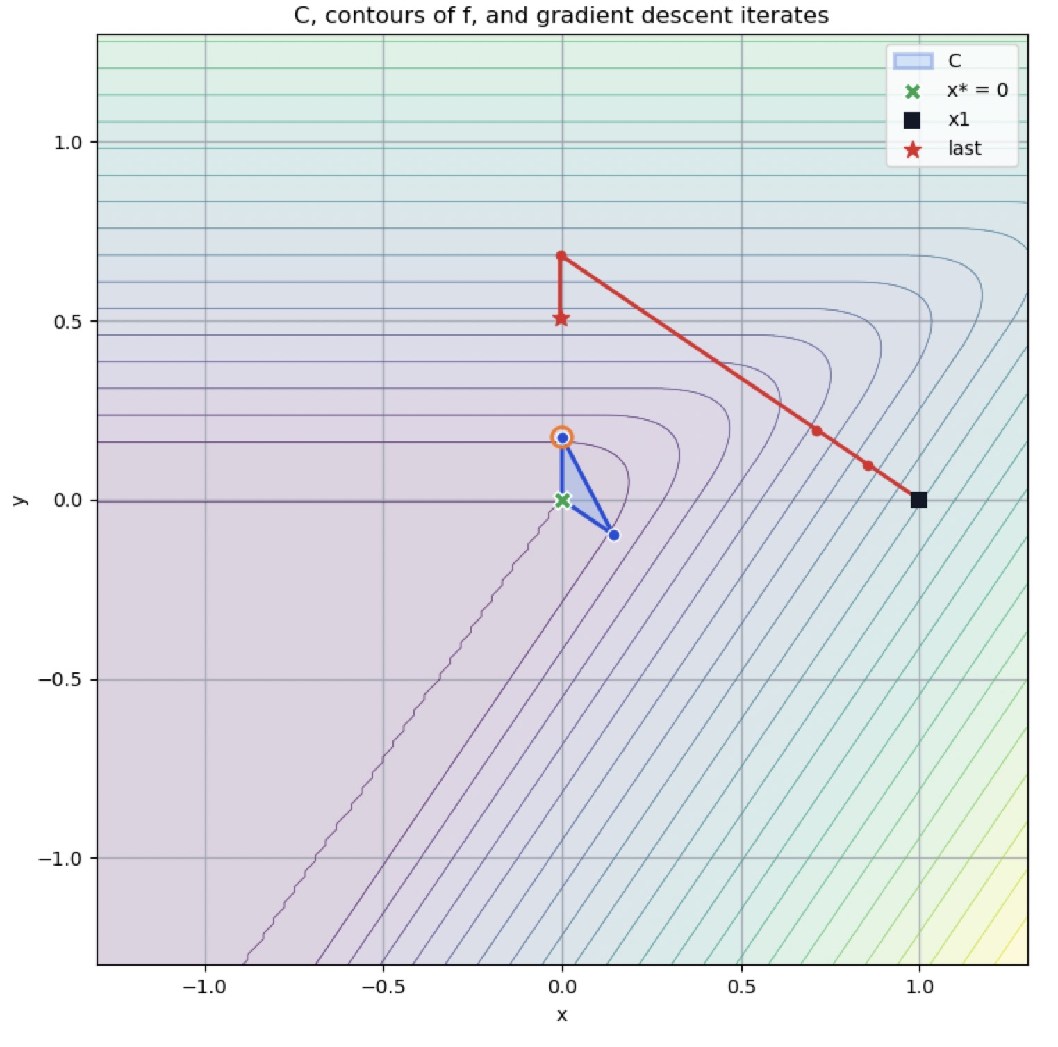
Let \( \{e_1,\ldots, e_{m+1}\} \) be the standard basis of \(\mathbb{R}^{m+1}\). We let \( x_1 = e_1 \) and construct \(C\subseteq\mathbb{R}^{m+1}\) such that GD has the following trajectory:
- For all \(i\in[m]\cup\{0\}\), we require \(x_{t_i+1}=\lambda_{i+1}e_{i+1}\) for some \(\lambda_{i+1}>0\). In other words, after the \(i\)-th large stepsize, the iterate lies on the \((i+1)\)-th axis. For the last iterate, we require \(x_{n+1}=\tau e_{m+1}\) for some \(\tau>0\).
- For all \(i\in[m]\) and \(t_{i-1}<k\leq t_i\), the iterates have the same gradient \(g_i\). For \(t_m<k\leq n\), the iterates have the same gradient \(g_{m+1}\). Therefore, between two large stepsizes, the trajectory of GD is a segment.
- Since the gradients of the generalized Huber functions (1) are the orthogonal projections, we let \(C = \text{conv}\{ 0, g_1,\ldots, g_{m+1} \}\).
These requirements impose sparsity of the iterates and the gradients which simplify the construction. At the same time, the constructed functions remain hard enough for GD. A simple example is given below:
Given these properties, we can derive the following necessary conditions on the gradients \(\{g_i\}\): $$g_i=\frac{1}{S_i+h_{t_i}}(\lambda_i e_i-\lambda_{i+1}e_{i+1}),\quad \forall i\in[m], \quad g_{m+1}=\frac{\lambda_{m+1}-\tau}{S_{m+1}}e_{m+1}.$$ Also, we can show that $$\tag{2} R_n \geq f(x_{n+1}) = 2\cdot\frac{\lambda_{m+1}-\tau}{S_{m+1}}\cdot\tau - \left(\frac{\lambda_{m+1}-\tau}{S_{m+1}}\right)^2.$$ It remains to find constraints on \(\{\lambda_i\}\) and \(\tau\) to ensure \(\Pi_C(x_k) = g_k\) for all \(i\in[m]\) and \(t_m<k\leq n\). Finally, we prove the lemma by maximizing (2) subject to these constraints.
Properties of Good Stepsize Schedules
Conditions on the Top-m Stepsizes
To make full use of Lemma 6, we want to choose \(m\) and the time indices \(\{t_i\}\) that maximize the lower bound. A natural choice is to select \(\{t_i\}\) to be the indices of the top-\(m\) largest stepsizes in \(H\). However, the resulting bound is still complicated, as it depends on the indices of the selected stepsizes. To further simplify the bound, Ma and Chen applied AM-GM inequalities to eliminate the dependence on the indices. The next lemma combines their approach with my further simplifications.
Lemma 7. (Top-\(m\) stepsizes) Fix any \(n\in\mathbb{N}\) and any \(H\in(0,\infty)^n\). Order the stepsizes as $$h^{\text{ord}}_1 \geq h^{\text{ord}}_2 \geq \cdots \geq h^{\text{ord}}_n.$$ For any \(m\in[n]\) such that \(h^{\text{ord}}_m>1\), let
- \(H_m:=( \frac{1}{m}\sum_{k=1}^m \frac{1}{h^{\text{ord}}_k-1} )^{-1}\) be the harmonic mean of \(\{ h_k^{\text{ord}} - 1 \}_{k\in[m]}\), and
- \(A_m:= h^{\text{ord}}_{m+1:n}\) be the sum of the remaining stepsizes.
Then, we have $$R_n(H) \geq \frac{(\gamma_m)^{m+1}}{24(A_m + m + 1)}, \quad \gamma_m := \frac{(m+1)H_m}{2(A_m + m + 1 + H_m)}.$$
Note that Lemma 7 depends only on the distribution of the stepsizes. Roughly speaking, it increases with the harmonic mean of the top-\(m\) stepsizes and decreases with the arithmetic mean (the sum) of the remaining small stepsizes. The proof of Lemma 7 is tedious and contains little insight, so I omit the details here.
Upper Bound on the Number of Large Stepsizes
Lemma 7 naturally leads to an upper bound on the number of large stepsizes. For any \(t\geq 1\), let $$N(t) := \lvert \{ k\in[n]: h_k \geq t \} \rvert$$ be the number of stepsizes greater than or equal to \(t\). We have the following lemma.
Lemma 8 (Number of large stepsizes) Let \(p=\sqrt{3}\). Fix any \(n\in\mathbb{N}\) and any \(H\in(0,\infty)^n\) such that \(R_n(H)\leq\frac{1}{24(3n+1)}\). For any \(t\geq 2\) such that $$\tag{3}\int_2^t N(s)\,\mathrm{d} s \leq \frac{1}{24R_n(H)} - (3n+1),$$ we have $$\tag{4}N(t)\leq\frac{5}{3} + \frac{2n}{(t-1)^{1/p}}.$$ The condition (3) can be replaced by $$\tag{5} \frac{5}{3}t+5nt^{1-1/p} \leq \frac{1}{24R_n(H)}-(3n+1). $$
If condition (3) holds, then the integral \(\int_2^t N(s)\,\mathrm{d} s\) is small, which means that the number of stepsizes below \(t\) is small. Therefore, Lemma 8 says that if, for some threshold \(t\), the number of stepsizes below \(t\) is small, then the number of large stepsizes exceeding \(t\) is also small.
Compared with Lemma 2.2 of Tsai et al., which shows that \(N(t)\lesssim nt^{-1/2} + \log n\) for all \(t\), Lemma 8 improves the upper bound when \(t\) satisfies the condition (3). A limitation of Lemma 8 is that it does not give any upper bound on \(N(t)\) when \(t\) is so large that the conditions (3) or (5) fails. Nevertheless, when they fail, they already provide lower bounds on \(R_n(H)\).
We start with Lemma 7. The idea is that if \(m\) is large, then we must have \(\gamma_m \leq 1\). Otherwise, if \(\gamma_m>1\), then \(\gamma_m^{m+1}\) grows exponentially in \(m\) and cannot be bounded by \(R_n(H)\). The condition \(\gamma_m\leq 1\) is equivalent to $$ H_m\leq\frac{2}{m-1}(A_m+m+1), $$ that is, the harmonic mean of the top-\(m\) stepsizes is controlled by the small stepsizes. If \(H_m\) is large, then \(m\) needs to be small. This implies an upper bound on the number of large stepsizes. In the following, we will let \(m=N(t)\) for \(t\geq1\). Note that \(m=N(t)\) increases as \(t\) decreases.
Suppose the condition (3) holds. By Lemma 7 and the layer-cake representation, we can show that $$ \begin{split} \left(\gamma_{N(t)}\right)^{N(t)+1} &\leq 24R_n(H)(A_{N(t)}+N(t)+1) \\ &\leq 24R_n(H)\left( \int_2^t N(s)\,ds+3n+1 \right). \end{split} $$ Combining the above inequality with (3) yields \(\gamma_{N(t)} \leq 1\). Note that since the left-hand side of (3) is increasing in \( t \), we also have \(\gamma_{N(s)} \leq 1\) for all \( s\in[2,t] \).
By using the layer-cake representation again, the condition \(\gamma_{N(t)} \leq 1\) is equivalent to the following quadratic inequality in \(N(t)\): $$\tag{6} \frac{N(t)(N(t)-1)}{2} \leq (U(t)-N(t))(N(t)-V(t)), $$ where \( U(t):=\frac{1}{t-1}\left(\int_0^t N(u)\,du+1\right) \) and \( V(t):=(t-1)\int_t^\infty\frac{N(u)}{(u-1)^2}\,du \). Solving this inequality for \(N(t)\) and simplifying the resulting bound gives \( N(t) \leq \frac{1}{3}(1+2W(t))\), where \(W(t) := U(t) + V(t)\).
Finally, we derive an upper bound on \(W(t)\). It can be verified that \( (s-1)W'(s) = V(s) - U(s) \) for almost all \( s\in [2, t] \). In the following, we show that \(V(t)-U(t)<-\rho W(t)+\tau\) for some \(\rho>0\) and \(\tau\geq0\). For any \(\rho\in(0,1)\), by the AM-GM inequality, $$ \begin{split} &-\rho W(s)-(V(s)-U(s))\\ &\qquad= (1-\rho)(U(s)-N(s))+(1+\rho)(N(s)-V(s))-2\rho N(s)\\ &\qquad\geq 2\sqrt{(1-\rho^2)(U(s)-N(s))(N(s)-V(s))}-2\rho N(s)\\ &\qquad\overset{(6)}{\geq} \sqrt{2(1-\rho^2)N(s)(N(s)-1)}-2\rho N(s). \end{split} $$ The last term is nonnegative if and only if $$ \rho\leq\sqrt{\frac{N(s)-1}{3N(s)-1}}. $$ Since the bound on \(\rho\) is approximately \(1/p\) when \(N(s)\) is large, we take \(\rho=1/p\). Since \(1-\rho^2=2\rho^2\), we have $$ -\rho W(s)-(V(s)-U(s)) \geq -2\rho\left(N(s)-\sqrt{N(s)(N(s)-1)}\right) \geq -2\rho, $$ where the second inequality follows from \(z-\sqrt{z(z-1)}\leq1\) for every \(z\geq1\). To conclude, we have \((W(s)-2)'\leq\frac{-\rho}{s-1}(W(s)-2) \) for all \( s\in[2,t]\). By Grönwall's inequality, $$ W(t)\leq 2+\frac{W(2)-2}{(t-1)^\rho}. $$ The proof of (4) follows from upper-bounding \(W(2)\). The condition (5) is obtained by using (4) to bound (3).
Proof of Theorem 2
Let \(p=\sqrt{3}\). Assume \( R_n(H)\leq\frac{1}{24(3n+1)}\). Otherwise, we have \(R_n(H)=\Omega(n^{-p})\) and the proof is complete. Pick \(t_0 = \Theta(n^p) \geq2\) such that the upper bound on \(N(t)\) in (4) of Lemma 8 is less than \(2\). We split the proof into two cases depending on whether \(t_0\) satisfies (5) in Lemma 8.
- Case 1: Suppose \(t_0\) does not satisfy (5) in Lemma 8. Then $$\frac53t_0+5nt_0^{1-1/p}>\frac{1}{24R_n(H)}-(3n+1),$$ which implies \( R_n(H) \gtrsim n^{-p} \).
- Case 2: Suppose \(t_0\) satisfies (5) in Lemma 8. Then for every \(t\in[2,t_0]\), $$ N(t)\leq\frac53+\frac{3n}{(t-1)^{1/p}}. $$ In particular, \(N(t_0)<2\) by the choice of \(t_0\), so \(N(t_0)\leq1\). Therefore, except for the largest stepsize, which we have no control over, all other stepsizes are less than \(t_0\). By the layer-cake representation and Lemma 8, we can show that \( A_1 \lesssim n^p \). Now we lower bound \(R_n(H)\) by \(A_1\). Let \(h^\star\) be the largest stepsize. If \(h^\star\gtrsim A_1\), then by Lemma 7 with \(m=1\), $$ R_n(H) \gtrsim \frac{1}{A_1}\left(\frac{h^\star-1}{A_1+h^\star+1} \right)^2 \gtrsim A_1^{-1}.$$ Otherwise, if \(h^\star \lesssim A_1\), by Lemma 3, $$R_n(H) \gtrsim \frac{1}{h_{1:n}} = \frac{1}{2A_1+2h^\star+1} \gtrsim A_1^{-1}.$$
Hence, regardless of the value of \(h^\star\), \( R_n(H) \gtrsim A_1^{-1} \). This completes the proof.
Concluding Remarks
The construction in Lemma 6 is very clever in my opinion. One particular question for which I do not have a satisfactory answer is why the current exponent of the lower bound is \(p=\sqrt{3}\). This number appears in the proof of Lemma 8, but I currently do not have a good interpretation of its role. Therefore, it is unclear to me whether \(p\) is the best exponent we can obtain from Lemma 6, or whether it is merely an artifact of our analysis. I would appreciate comments or insights on this point.
Bibliographic Information
@misc{tsai2026,
  author = {Chung-En Tsai},
  title = {An Improved Lower Bound for Non-Anytime Gradient Descent},
  year = {2026},
  note = {Blog post},
  url = {https://chungentsai.github.io/gd-lower-bounds.html}
}