Online Portfolio Selection
Introduction
Suppose that we are investing in a market with \(d\) stocks. But we do not have any information about the market. We don't know whether the prices follow any probability distributions. How should we distribute our money every day in order to make our wealth grow as much as possible? Online portfolio selection (OPS) provides a simple and clean framework to study the investment problem.
OPS was proposed by Thomas M. Cover thirty years ago [1]. OPS models the investment as a multi-round game between two players, named Investor and Market. The game proceeds as follows.
Protocol: On the \(t\)-th day (\(t=1,2,3,\ldots\)),
- Investor chooses a portfolio \(x_t\in\Delta\subseteq\mathbb{R}^d\).
- Market observes \(x_t\) and announces a vector of price relatives \(r_t\in[0,\infty)^d\).
- Investor's wealth grows by a ratio of \(\langle r_t, x_t\rangle\).
Explanation of the protocol
How should we measure Investor's performance? Note that Market chooses \(r_t\) after observing \(x_t\), so it is impossible for Investor to earn money in this game. Therefore, the "absolute" magnitude of Investor's wealth after \(T\) days is not an appropriate performance measure. Cover considered the ratio of the highest wealth obtained by some investment strategies to Investor's wealth. More precisely, he considered to design Investor's strategy to minimize the wealth ratio $$ \frac{ \max_{x\in\Delta} \prod_{t=1}^T \langle r_t, x\rangle }{ \prod_{t=1}^T \langle r_t, x_t \rangle }, $$ where the numerator is the highest possible wealth obtained by the so-called constantly rebalanced portfolios and the denominator is Investor's wealth. A question left here is: is minimizing this ratio a meaningful goal for Investor?
In the literature, the above goal usually appears in an equivalent form. That is, minimizing the regret, which is the logarithm of the wealth ratio: $$ R_T(r_1,\ldots,r_T) := \sum_{t=1}^T -\log\langle r_t, x_t \rangle - \min_{x\in\Delta} \sum_{t=1}^T -\log\langle r_t, x\rangle. $$
Besides being an investment problem, OPS is a classical problem in the field of online learning. For example, see Chapter 10 of Prediction, Learning, and Games [2] and Chapter 12 of Orabona's lecture notes [3]. OPS algorithms can also be used to solve the Poisson inverse problem [4], which has applications in medical imaging or astronomical denoising.
Existing Algorithms

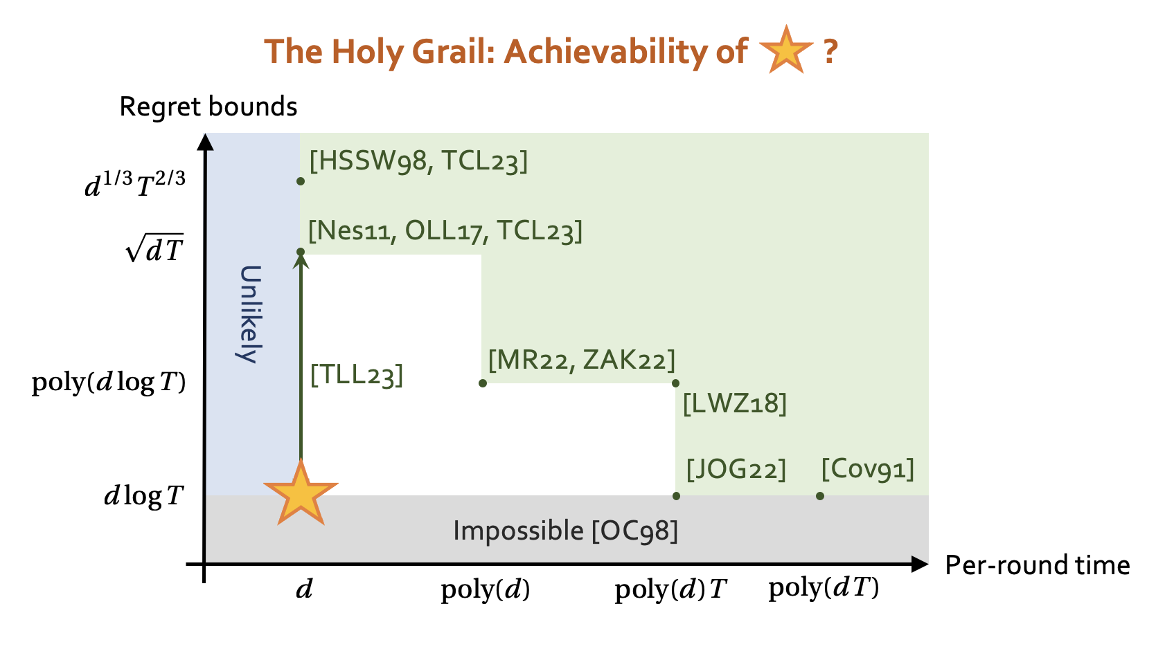
The first paper using the term "Pareto frontier" in OPS is the work of Zimmert et al. [5].
| Algorithms | Regret (\(\tilde{O}\)) | Per-round time (\(\tilde{O}\)) |
|---|---|---|
| Universal Portfolio [1, 7] | \(d\log T\) | \(d^4T^{14}\) |
| \(\widetilde{\text{EG}}\) [8, 9] | \(d^{1/3}T^{2/3}\) | \(d\) |
| Barrier subgradient method [10] | \( \sqrt{dT} \) | \(d\) |
| Soft-Bayes [11] | \( \sqrt{dT} \) | \( d \) |
| LB-OMD [9] | \( \sqrt{dT} \) | \( d \) |
| ADA-BARRONS [12] | \( d^2\log^4T \) | \( d^{2.5}T \) |
| LB-FTRL without linearized losses [13] | \( d\log^{d+1}T \) | \( d^2T \) |
| PAE+DONS [14] | \( d^2\log^5T \) | \( d^3 \) |
| BISONS [5] | \( d^2\log^2 T \) | \( d^3 \) |
| VB-FTRL [15] | \( d\log T \) | \( d^2T \) |
| Adaptive LB-FTRL [16] | \( d\log^2 T \) ~ \( \sqrt{dT} \) | \( d \) |
| Optimistic LB-FTRL [16] | \( d\log T \) ~ \( \sqrt{dT} \) | \( d \) |
References
- T. M. Cover. "Universal portfolios." Math. Financ. 1991.
- N. Cesa-Bianchi and G. Lugosi. Prediction, Learning, and Games. Cambridge University Press. 2006.
- F. Orabona. "A modern introduction to online learning." arXiv preprint arXiv:1912.13213v6. 2023.
- Y.-H. Li. "Online positron emission tomography by online portfolio selection." ICASSP 2020.
- J. Zimmert, N. Agarwal, and S. Kale. "Pushing the efficiency-regret Pareto frontier for online learning of portfolios and quantum states." COLT 2022.
- E. Ordentlich and T. M. Cover. "The cost of achieving the best portfolio in hindsight." Math. Oper. Res. 1998.
- A. Kalai and S. Vempala. "Efficient algorithms for universal portfolios." J. Mach. Learn. Res. 2002.
- D. P. Helmbold, R. E. Schapire, Y. Singer, and M. K. Warmuth. "On-line portfolio selection using multiplicative updates." Math. Financ. 1998.
- C.-E. Tsai, H.-C. Cheng, and Y.-H. Li. "Online self-concordant and relatively smooth minimization, with applications to online portfolio selection and learning quantum states." ALT 2023
- Y. Nesterov. "Barrier subgradient method." Math. Program. 2010.
- L. Orseau, T. Lattimore, and S. Legg. "Soft-Bayes: prod for mixtures of experts with log-loss." ALT 2017.
- H. Luo, C.-Y. Wei, and K. Zheng. "Efficient online portfolio with logarithmic regret." NeurIPS 2018.
- T. van Erven, D. van der Hoeven, W. Kotłowski, and W. M. Koolen. "Open problem: fast and optimal online portfolio selection." COLT 2020.
- Z. Mhammedi and A. Rakhlin. "Damped online Newton step for portfolio selection." COLT 2022.
- R. Jézéquel, D. M. Ostrovskii, and P. Gaillard. "Efficient and near-optimal online portfolio selection." arXiv preprint arXiv:2209.13932. 2022.
- C.-E. Tsai, Y.-T. Lin, and Y.-H. Li. "Data-dependent bounds for online portfolio selection without Lipschitzness and smoothness." NeurIPS 2023.